A recent paper of mine proposed an algorithm to do weakly-supervised inverse RL from goal states (check out the paper!). The algorithm is derived through an interesting framework called "control as inference", which analogizes (max-ent) reinforcement learning as inference in a graphical model. This framework has been gaining traction recently, and it's been used to justify many recent contributions in IRL (Finn et al, Fu et al), and some interesting RL algorithms like Soft Q-Learning(Haarnoja et al).
I personally think the framework is very cute, and it's an interesting paradigm which can explain some weird quirks that show up in RL. This document is a writeup which explains exactly what "control as inference" is. Once you've finished reading this, you may also enjoy this lecture in Sergey Levine's CS294-112 class, or his primer on control as inference as a more detailed reference.
The MDP
In this article, we'll focus on a finite-horizon MDP with horizon $T$ : this is simply for convenience, and all the derivations and proofs can be extended to the infinite horizon case simply. Recall that an MDP is $(\mathcal{S}, \mathcal{A}, \mathcal{T}, \rho, R)$ , where $\mathcal{S,A}$ are the state and action spaces, $T(\cdot \vert s,a)$ is the transition kernel, $\rho$ the initial state distribution, and $R$ the reward.
The Graphical Model
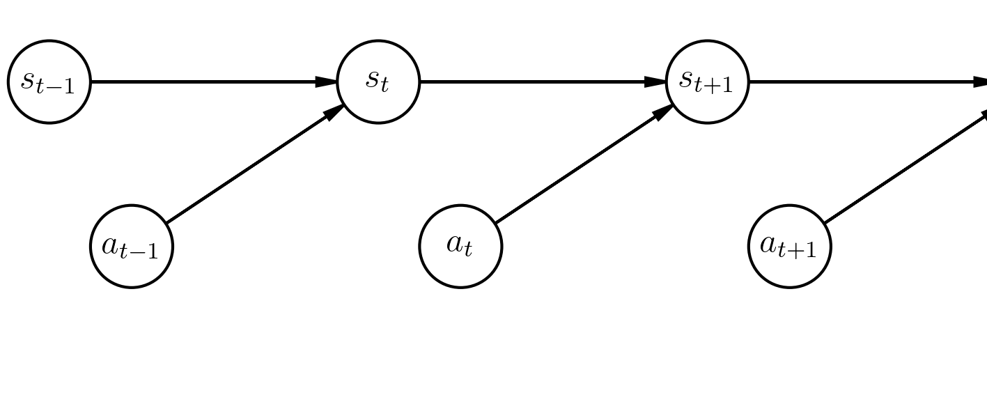
Trajectories in an MDP as detailed above can be modelled by the following graphical model.

The graphical model has a state variable $S_t$, an action variable $A_t$ for each timestep $t$.
We'll define the distributions of the variables in this graphical model in a way such that the probability of a trajectory $\tau = (s_0, a_0, s_1, a_1, \dots s_T)$ is equal to the probability of the trajectory under the MDP's dynamics.
We set the distribution of $S_0$ to be $\rho(s)$ (the initial state distribution of the MDP).
For subsequent $S_{t}$, the distribution is defined using transition probabilities of the MDP.
$$P(S_{t+1} = s' \vert S_{t}=s, A_t = a) = T(s' \vert a,s)$$The distribution for the action variables $A_t$ is uniform on the action space.
$$P(A_t = a) = C$$It may seem odd that the actions are sampled uniformly, but don't worry! These are only prior probabilities, and we'll get interesting action distributions once we start conditioning (Hang tight!)
The probability of a trajectory $\tau = (s_0, a_0, s_1, a_1 , \dots s_T,a_T)$ in this model factorizes as
$$\begin{align*}P(\tau) &= P(S_0 = s_0) \prod_{t=0}^{T-1} P(A_t = a_t)P(S_{t+1} = s_{t+1} | S_t = s_t, A_t = a_t)\\ &= C^T \left(\rho(s_0) \prod_{t=0}^{T-1} T(s_{t+1} \vert s_t, a_t)\right)\\ &\propto \left(\rho(s_0)\prod_{t=0}^{T-1} T(s_{t+1} | s_t,a_t)\right) \end{align*}$$The probability of a trajectory in our graphical model is thus directly proportional to the probability under the system dynamics.
In the special case that dynamics are deterministic, then $P(\tau) \propto \mathbb{1} \{\text{Feasible}\}$ (that is, all trajectories are equally likely).
Adding Rewards
So far, we have a general structure for describing the likelihood of trajectories in an MDP, but it's highly uninteresting since at the moment, all trajectories are equally likely. To highlight interesting trajectories, we'll introduce the concept of optimality.
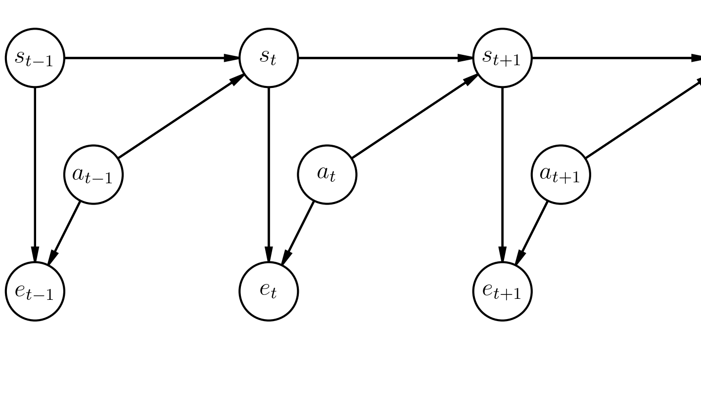
We'll say that an agent is optimal at timestep $t$ with some probability which depends on the current state and action : $P(\text{Optimal at } t) = f(s_t,a_t)$. We'll embed optimality into our graphical model with a binary random variable at every timestep $e_t$, where $P(e_t = 1 \vert S_t=s_t, A_t=a_t) = f(s_t,a_t)$.
While we're at it, let's define a function $r(s,a)$ to be $r(s_t,a_t) = \log f(s_t,a_t)$ . The notation is very suggestive, and indeed we'll see very soon that this function $r(s,a)$ plays the role of a reward function.
The final graphical model, presented below, ends up looking much like one for a Hidden Markov Model.

For a trajectory $\tau$, the probability that it is optimal at all timesteps is proportional (exponentially) to the total reward received in the trajectory.
$$P(\text{All } e_t=1 | \tau) =\exp (\sum_{t=0}^T r(s_t,a_t))$$$$\begin{align*}P(\text{All } e_t=1 | \tau) &= \prod_{t=0}^T P(e_t = 1 \vert S_t=s_t, A_t=a_t) \\ &= \prod_{t=0}^T f(s_t,a_t) \\ &= \prod_{t=0}^T \exp{r(s_t,a_t)} \\ &= \exp (\sum_{t=0}^T r(s_t,a_t))\end{align*}$$
We'll describe the optimal trajectory distribution as the distribution when conditioned on being optimal at all time steps. $$\pi_{\text{optimal}}(\tau) = P(\tau \vert \text{All } e_t =1) = P(\tau~\vert~e_{1:T} = 1)$$
Explicitly writing out this distribution, we have that
$$P(\tau ~\vert ~e_{1:T} = 1) \propto \exp(\sum_{t=0}^T r(s_t,a_t))P(\tau)$$$$\begin{align*}P(\tau ~\vert~ e_{1:T} =1) &= \frac{P(e_{1:T} =1 \vert \tau)P(\tau)}{P(e_{1:T} =1)} \\ &\propto P(e_{1:T} =1 \vert \tau)P(\tau) \\ &\propto \exp(\sum_{t=0}^T r(s_t,a_t))P(\tau)\end{align*}$$
Under deterministic dynamics, since $P(\tau) \propto \mathbb{1}\{\text{Feasible}\}$, the probability of any feasible trajectory is $$P(\tau~\vert~ e_{1:T} =1) \propto \exp(\sum_{t=0}^T r(s_t,a_t))$$
This can be viewed as a special form of an energy-based model, where the energy of a trajectory is proportional to the reward.
Exact Inference in the Graphical Model
We now have a model for what the optimal trajectory distribution is, so the next appropriate step is to look at optimal action distributions. If I am at state $s$ on timestep $t$, what is the "optimal" distribution of actions?
Pedantically, this corresponds to finding $$\pi_{t}(a \vert s) = P(A_t = a~\vert~S_t = s,e_{1:T} =1)$$
In our graphical model, $A_t$ is independent of all events before $t$ ($A_t \perp E_1 \dots E_{t-1})$. We can verify this mathematically, but the intuition is that the distribution of actions at a timestep shouldn't be impacted by what happened previously (the environment is Markovian). So,
$$\pi_{t}(a \vert s) = P(A_t = a \vert S_t = s, e_{t:T} =1)$$Solving for these probabilities corresponds to doing exact inference in the graphical model above, which looks much like the forward-backward algorithm for HMMs. The procedure goes as follows:
- Backward message passing: Compute probabilities $P(e_{t:T} = 1 ~\vert~ S_t =s)$ and $P(e_{t:T} = 1 ~\vert~ S_t =s, A_{t} = a)$
- Forward message passing: Compute probabilities $P(A_t = a \vert S_t = s, e_{t:T} =1)$ using Bayes Rule and the backwards messages.
Backward Messages
We can compute these backward messages recursively, since
- $P(e_{t:T} = 1\vert A_t =a, S_t=s)$ can be expressed in terms of $P(e_{t+1:T} = 1 \vert S_{t+1} = s')$
- $P(e_{t:T} = 1\vert S_t=s)$ can be expressed in terms of $P(e_{t:T} = 1\vert S_t=s, A_t =a)$
Working through the math (see the proof for more details)
$$P(e_{t:T} = 1 = e^{r(s,a)} \mathbb{E}_{s' \sim T(\cdot \vert s,a)}[P(e_{t+1:T}=1 \vert S_{t+1}=s')]$$
$$P(e_{t:T} = 1\vert S_t=s) = \mathbb{E}_{a}[P(e_{t:T} = 1 \vert A_t=a, S_t =s)]$$
$$ \begin{align*} P(e_{t:T} = 1&\vert A_t =a, S_t=s)\\ &= \int_{\mathcal{S}} P(e_{t:T}=1, S_{t+1}=s' \vert S_t=s, A_t=a) ds'\\ &= \int_{\mathcal{S}} P(e_t = 1 | S_t=s, A_t=a)P(e_{t+1:T}=1, S_{t+1}=s' \vert S_t=s, A_t=a) ds'\\ &= P(e_t = 1 | S_t=s, A_t=a) \int_{\mathcal{S}} P(e_{t+1:T}=1 \vert S_{t+1}=s') P(S_{t+1} = s' \vert S_t=s, A_t=a) ds'\\ &= e^{r(s,a)} \mathbb{E}_{s' \sim T(\cdot \vert s,a)}[P(e_{t+1:T}=1 \vert S_{t+1}=s')]\\ P(e_{t:T} = 1&\vert S_t=s)\\ &= \int_{\mathcal{A}} P(e_{t:T} = 1, A_t=a \vert S_t=s) da\\ &= \int_{\mathcal{A}} P(e_{t:T} = 1 \vert A_t=a , S_t=s) P(A_t=a) da \\ &= \mathbb{E}_{a}[P(e_{t:T} = 1 \vert A_t=a, S_t =s)]\\ \end{align*} $$
That looks pretty ugly and uninterpretable, but if we view the expressions in log-probability space, there's rich meaning.
Let's define $$Q_t(s,a) = \log P(e_{t:T} = 1\vert A_t =a, S_t=s)$$ $$V_t(s) = \log P(e_{t:T} = 1 \vert S_t=s)$$
$Q$ and $V$ are very suggestively named for a good reason: we'll discover that they are the analogue of the $Q$ and $V$ functions in standard RL. Rewriting the above expressions with $Q_t(\cdot, \cdot)$ and $V_t(\cdot)$:
$$Q_t(s,a) = r(s,a) + \log \mathbb{E}_{s' \sim T(\cdot \vert s,a)}[e^{V_{t+1}(s')}]$$$$V_t(s) = \log \mathbb{E}_a [e^{Q_t(s,a)}]$$Remember that the function $\log \mathbb{E}[\exp(f(X))] $ acts as a "soft" maximum operation: that is $$\log \mathbb{E}[\exp(f(X))] = \text{soft} \max_X f(X) \approx \max_{X} f(X)$$
We'll denote it as $\text{soft} \max$ from now on - but don't get it confused with the actual softmax operator. With this notation:
$$Q_t(s,a) = r(s,a) + \text{soft} \max_{s'} V_{t+1}(s')$$$$V_t(s) = \text{soft} \max_{a} Q_{t}(s,a)$$These recursive equations look very much like the Bellman backup equations!
These are the soft Bellman backup equations. They differ from the traditional Bellman backup in two ways:
- The value function is a "soft" maximum over actions, not a hard maximum.
- The q-value function is a "soft" maximum over next states, not an expectation: this makes the Q-value "optimistic wrt the system dynamics" or "risk-seeking". It'll favor actions which have a low probability of going to a really good state over actions which have high probability of going to a somewhat good state. When dynamics are deterministic, then the Q-update is equivalent to the normal backup: $Q_t(s,a) = r(s,a) + V_{t+1}(s')$.
Passing backwards messages corresponds to performing Bellman updates in an MDP, albeit with slightly different backup operations
Forward Messages
Now that we know that the $Q$ and $V$ functions correspond to backward messages, let's now compute the optimal action distribution.
$$ \begin{align*} P(A_t =a \vert S_t=s, e_{t:T}=1) &= \frac{P(e_{t:T}=1 \vert A_t =a, S_t=s)P(A_t = a \vert S_t =s)}{P(e_{t:T}=1\vert S_t=s)}\\ &= \frac{e^{Q_t(s,a)}C}{e^{V_t(s)}}\\ &\propto \exp(Q_t(s,a) - V_t(s))\\ &\propto \exp(A_t(s,a)) \end{align*} $$If we define the advantage $A_t(s,a) = Q_t(s,a) - V_t(s)$, then we find that the optimal probability of picking an action is simply proportional to the exponentiated advantage!
Haarnoja et al perform a derivation similar to this to find an algorithm called Soft Q-Learning. In their paper, they show that the soft bellman backup update is a contraction, and so Q-learning with the soft backup equations have the same convergence guarantees that Q-learning has in the discrete case. Empirically, they show that this algorithm can learn complicated continuous control tasks with high sample efficiency. In follow-up works, they deploy the algorithms on robots and also present actor-critic methods in this framework.
Approximate Inference with variational methods
Let's try to look at inference in this graphical model in a different way. Instead of doing exact inference in the original model to get a policy distribution, we can attempt to learn a variational approximation to our intended distribution $q_{\theta}(\tau) \approx P(\tau \vert e_{1:T}=1)$.
The motivation is the following: we want to learn a policy $\pi(a \vert s)$ such that sampling actions from $\pi$ causes the trajectory distribution to look as close to $P(\tau \vert e_{1:T} = 1)$ as possible. We'll define a variational distribution $q_{\theta}(\tau)$ as follows:
$$q_\theta(\tau) = P(S_0 = s_0) \prod_{t=0}^T q_{\theta}(a_t \vert s_t) P(S_{t+1} = s_{t+1} \vert S_{t} = s_t, A_t = a_t) = \left(\prod_{t=0}^T q(a_t | s_t)\right) P(\tau)$$This variational distribution can change the distribution of actions, but fixes the system dynamics in place. This is a form of structured variational inference, and we attempt to find the function $q_{\theta}(a \vert s)$ which minimizes the KL divergence with our target distribution.
$$\min_{\theta} D_{KL}(q_{\theta}(\tau) \| P(\tau \vert e_{1:T} = 1))$$If we simplify the expressions, it turns out that
$$\arg\min_{\theta} D_{KL}(q_{\theta}(\tau) \| P(\tau \vert e_{1:T} = 1)) = \arg \max_{\theta} \mathbb{E}_{\tau \sim q}[ \sum_{t=0}^T r(s_t,a_t) + \mathcal{H}(q_{\theta}(\cdot \vert s_t)]$$Remember from the first section that $P(\tau \vert \text{All } e_t=1) = P(\tau) \exp(\sum_{t=0}^T r(s_t,a_t))$ $$ \begin{align*} D_{KL}(q_{\theta}(\tau) \| P(\tau \vert \text{All } e_t = 1)) &= -\mathbb{E}_{\tau \sim q}[\log \frac{P(\tau \vert \text{All } e_t = 1)}{q_{\theta}(\tau)}]\\ &= -\mathbb{E}_{\tau \sim q}[\log \frac{P(\tau) \exp(\sum_{t=0}^T r(s_t,a_t))}{ P(\tau)\left(\prod_{t=0}^T q_{\theta}(a_t | s_t)\right)}]\\ &= -\mathbb{E}_{\tau \sim q}[\log \frac{\exp(\sum_{t=0}^T r(s_t,a_t))}{\prod_{t=0}^T q_{\theta}(a_t | s_t)}]\\ &= -\mathbb{E}_{\tau \sim q}[\log \frac{\exp(\sum_{t=0}^T r(s_t,a_t))}{\exp (\sum_{t=0}^T \log q_{\theta}(a_t | s_t)}]\\ &= -\mathbb{E}_{\tau \sim q}[ \sum_{t=0}^T r(s_t,a_t) - \log q_{\theta}(a_t | s_t))]\\ \end{align*} $$ Recalling that $-\log q(a_t | s_t)$ is a point estimate of the entropy of $q_{\theta}$: $\mathcal{H}(q(\cdot \vert s))$, we get our result.
$$D_{KL}(q_{\theta}(\tau) \| P(\tau \vert e_{1:T} = 1)) = -\mathbb{E}_{\tau \sim q}[ \sum_{t=0}^T r(s_t,a_t) + \mathcal{H}(q_{\theta}(\cdot \vert s_t)]$$The best policy $q_{\theta}(a|s)$ is thus the one that maximizes expected reward with an entropy bonus. This is the the objective for maximum entropy reinforcement learning. Performing structured variational inference with this particular family of distributions to minimize the KL divergence with the optimal trajectory distribution is equivalent to doing reinforcement learning in the max-ent setting!
Inferring Reward with Maximum Entropy Inverse Reinforcement Learning
To Be Continued
This tutorial is a work in progress. Stay tuned for more updates!