What is TensorFlow?
If you've been following the machine learning community, in particular that of deep learning, over the last year, you've probably heard of Tensorflow. Tensorflow is a library to structure and run numerical computations developed in-house by Google Brain (the people who developed Alpha-GO). One can imagine this library as an extension of NumPY to work on more scalable architectures, as well as with more detailed algorithms and methods that pertain specifically to machine learning. Tensorflow joins Theano and cuDNN as architectures for building and designing neural networks.
This article hopes to delve into Tensorflow through case studies of implementations of Neural Networks. As such, it requires advance knowledge of neural networks (the subject is too expansive to cover in a single article). For those new (and for those who need a refresher), here are some good reference materials
Installation
Tensorflow is available on PyPI, so we can simply pip install
pip install tensorflow
Or if you have a GPU
pip install tensorflow-gpu
More extensive installation details can be found on the Tensorflow Installation Website
How This Article Is Set Up
We follow the Theano Tutorials which build up from basic addition/multiplication all the way to convolutional neural networks
Initial Investigations
- Multiplication
- Linear Regression
- Logistic Regression
Neural Networks
- Fully-connected Feed-Forward Neural Network (FC NN)
- "Deep" Fully Connected Neural Network
- Convolutional Neural Network
First, let's get the default imports out of the way: these imports will be used throughout the guide, and others will be added later when necessary
import tensorflow as tf
import numpy as np
import matplotlib.pyplot as plt
%matplotlib inline
Multiplication
Given two floats $x$ and $y$, find $xy$
First we create the relevant variables x and y (initializing them as floats). Placeholders can be thought of as inputs; when doing computations, we'll plug in values for x and y. We symbolize the result that we are looking for as xy.
x = tf.placeholder("float")
y = tf.placeholder("float")
xy = tf.mul(x,y)
Now we've represented the computation graph in Tensorflow; all that remains is to create a session, and plug in values, retrieving the result of the computation
with tf.Session() as sess:
print("%f x %f = %f"%(2,3,sess.run(xy,feed_dict={x:2,y:3})))
2.000000 x 3.000000 = 6.000000
Linear Regression
Given $\{(x_1,y_1) \dots (x_n,y_n)\}$, find $w$ and $b$ such that it minimizes $$\sum (wx_i + b - y_i)^2$$
First, let's create some sample data to work with:
We model $y = 2x + \mathcal{N}(0,1)$ (there's some random noise)
trX = np.linspace(-1, 1, 500)
trY = 2 * trX + np.random.randn(*trX.shape)*.35 + 2
plt.scatter(trX,trY);
Here, we again define our inputs x and y again. We define a variable w which stores the weight; variables are objects in Tensorflow which we use to represent internal states and are updatable. Again y_hat is simply our prediction
X = tf.placeholder("float")
Y = tf.placeholder("float")
w = tf.Variable(0.0,name="weights")
b = tf.Variable(0.0, name="bias")
y_hat = tf.add(tf.mul(X,w),b)
Let's now define our cost model and the underlying optimizer. Here, we opt for the squared loss objective (there are many others similar).
In order to optimize the function over $w$ and $b$, we create a GD optimizer, and minimize over the given cost function. Here we set $\alpha = .01$ (the learning rate)
cost = tf.reduce_mean(tf.square(Y - y_hat))
train_operation = tf.train.GradientDescentOptimizer(.01).minimize(cost)
Now, we simply run the train_operation, passing in our input data (this is Gradient Descent , not SGD). Since we created variables (w and b), we need to initialize them in the session with tf.initialize_all_variables().run()
numEpochs = 200
costs = []
with tf.Session() as sess:
tf.initialize_all_variables().run()
for i in range(numEpochs):
sess.run(train_operation,feed_dict={X:trX,Y: trY})
costs.append(sess.run(cost,feed_dict={X:trX,Y: trY}))
print("Final Error is %f"%costs[-1])
wfinal,bfinal = sess.run(w),sess.run(b)
print("Predicting y = %.02f x + %.02f"%(wfinal,bfinal))
print("Actually is y = %.02f x + %.02f"%(2,2))
Final Error is 0.217815
Predicting  y = 1.52 x + 1.95
Actually is y = 2.00 x + 2.00
plt.plot(costs)
plt.ylabel("Mean Squared Error")
plt.xlabel("Epoch");
Let's try to expand this to the multivariable case, where $x \in \mathbb{R}^n$,$w \in \mathbb{R}^{n \times m}$, and where $y$ is modelled with gaussian noise as
$$ y = W^Tx + \mathcal{N}(0,I_m)$$
m = 8
n = 5
NUM_EXAMPLES = 100
W = np.random.rand(n,m)
trX = np.random.rand(100,n)
trY = X.dot(W) + np.random.randn(NUM_EXAMPLES,m)
trX.shape, trY.shape
We again define our x and y placeholder inputs similarly; however, this time we explicitly add a shape parameter to the data. The first None is the dimension of the batch-size (variable), and the second number our actual dimension.
x = tf.placeholder("float",shape=[None, n])
y = tf.placeholder("float",shape=[None, m])
w = tf.Variable(tf.zeros([n,m]))
y_hat = tf.matmul(x,w)
The rest remains the same
cost = tf.reduce_mean(tf.square(y - y_hat))
train_operation = tf.train.GradientDescentOptimizer(.01).minimize(cost)
numEpochs = 1000
costs = []
with tf.Session() as sess:
tf.initialize_all_variables().run()
for i in range(numEpochs):
sess.run(train_operation,feed_dict={x:trX,y: trY})
costs.append(sess.run(cost,feed_dict={x:trX,y: trY}))
print("Final Error is %f"%costs[-1])
plt.plot(costs)
plt.ylabel("Mean Squared Error")
plt.xlabel("Epoch");
We shall use the MNIST dataset for this example. Conveniently, Tensorflow has a library to read the MNIST files
from tensorflow.examples.tutorials.mnist import input_data
mnist = input_data.read_data_sets("MNIST/",one_hot=True)
trX, trY = mnist.train.images, mnist.train.labels
teX, teY = mnist.test.images, mnist.test.labels
Extracting MNIST/train-images-idx3-ubyte.gz
Extracting MNIST/train-labels-idx1-ubyte.gz
Extracting MNIST/t10k-images-idx3-ubyte.gz
Extracting MNIST/t10k-labels-idx1-ubyte.gz
Recall in logistic regression that we model the logit as a linear transformation of $x$, and perform MLE over $W$. Notice the MLE likelihood function is simply just the cross entropy on the logit of the linear model. Using this philosophy, we express our logistic model
X = tf.placeholder("float",shape=[None,784])
Y = tf.placeholder("float",shape=[None,10])
w = tf.Variable(tf.random_normal([784,10], stddev=0.01))
pred_logit = tf.matmul(X,w)
sample_cost = tf.nn.softmax_cross_entropy_with_logits(pred_logit,Y)
total_cost = tf.reduce_mean(sample_cost)
train_operation = tf.train.GradientDescentOptimizer(0.05).minimize(total_cost)
predict_operation = tf.argmax(pred_logit, 1)
accuracy_operation = tf.reduce_mean(
tf.cast(tf.equal(predict_operation,tf.argmax(Y,1)),tf.float32)
)
Let's train! We'll do batch gradient descent here to speed up training times
NUM_EPOCHS = 30
BATCH_SIZE = 200
accuracies = []
with tf.Session() as sess:
tf.initialize_all_variables().run()
for epoch in range(NUM_EPOCHS):
for start in range(0,len(trX),BATCH_SIZE):
end = start + BATCH_SIZE
sess.run(train_operation, \
feed_dict = {X: trX[start:end],Y: trY[start:end]})
accuracies.append(sess.run(accuracy_operation,feed_dict= {X: teX,Y: teY}))
plt.plot(accuracies)
Out[22]:
[<matplotlib.lines.Line2D at 0x7fd8dc56ce48>]
Before beginning the neural network section, we introduce some common code bases, which shall be shared by all the neural networks that follow. This allows us to abstract our code, and work in a cleaner environment. In particular, we define code to create variables (these are our parameters that we learn) initiated randomly, and code to train our model
import tqdm # Using this for dynamic updates instead of unwieldy print statements
import time # Timing how long it takes an epoch to run
def init_weights(shape):
return tf.Variable(tf.random_normal(shape,stddev=0.01))
def update_d(prev,new):
combined = prev.copy()
combined.update(new)
return combined
def train_model(sess,train_X,train_Y, test_X,test_Y,train_operation,accuracy_operation,num_epochs,batch_size,test_size,train_feed=dict(),test_feed=dict(),howOften=100):
accuracies = []
startingTime = time.time()
with tqdm.tqdm(total= num_epochs * len(train_X)) as ranger:
for epoch in range(num_epochs):
for start in range(0,len(train_X),batch_size):
end = start + batch_size
sess.run(train_operation, \
feed_dict = update_d(train_feed,{X: train_X[start:end],Y: train_Y[start:end]}))
ranger.update(batch_size)
if (start//batch_size)%howOften == 0:
testSet = np.random.choice(len(test_X),test_size,replace=False)
tX,tY = test_X[testSet],test_Y[testSet]
accuracies.append(sess.run(accuracy_operation,feed_dict= update_d(test_feed,{X: tX,Y: tY})))
ranger.set_description("Test Accuracy: " + str(accuracies[-1]))
testSet = np.random.choice(len(test_X),test_size,replace=False)
tX,tY = test_X[testSet],test_Y[testSet]
accuracies.append(sess.run(accuracy_operation,feed_dict= update_d(test_feed,{X: tX,Y: tY})))
ranger.set_description("Test Accuracy: " + str(accuracies[-1]))
timeTaken = time.time() - startingTime
print("Finished training for %d epochs"%num_epochs)
print("Took %.02f seconds (%.02f s per epoch)"%(timeTaken,timeTaken/num_epochs))
accuracies.append(sess.run(accuracy_operation,feed_dict= update_d(test_feed,{X: test_X,Y: test_Y})))
print("Final accuracy was %.04f"%accuracies[-1])
plt.plot(accuracies)
Basic Fully Connected Network
We shall use the "classic" starting neural network; which consists of the input layer, a hidden layer coupled with the sigmoid activation function, and finally an output layer, upon which we shall run softmax (paired with the cross-entropy loss). As in the previous example on logistic regression, the softmax won't be directly computed, and instead implicitly factored in through the cost function. We again shall train on the MNIST dataset
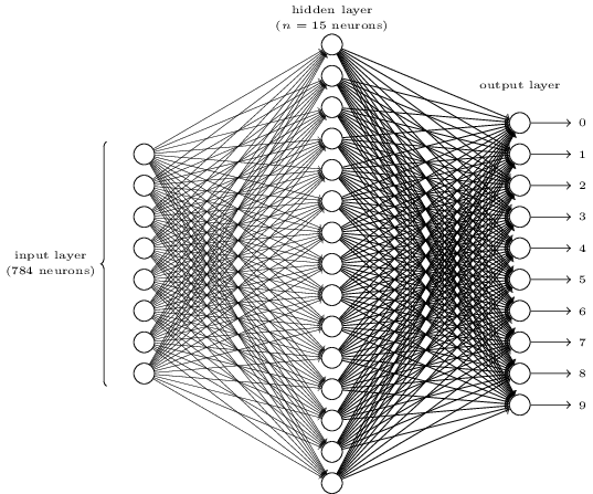
NUM_HIDDEN = 620
X = tf.placeholder("float",shape=[None,784])
Y = tf.placeholder("float",shape=[None,10])
def init_weights(shape): # We define this out of convenience
return tf.Variable(tf.random_normal(shape, stddev=0.01))
W_h = init_weights([784,NUM_HIDDEN]) # Weights entering the hidden layer
W_o = init_weights([NUM_HIDDEN,10]) # Weights entering the output layer
entering_hidden = tf.matmul(X,W_h)
exiting_hidden = tf.nn.sigmoid(entering_hidden)
model = tf.matmul(exiting_hidden,W_o)
sample_cost = tf.nn.softmax_cross_entropy_with_logits(model,Y)
total_cost = tf.reduce_mean(sample_cost)
train_operation = tf.train.GradientDescentOptimizer(0.2).minimize(total_cost)
predict_operation = tf.argmax(model, 1)
accuracy_operation = tf.reduce_mean(
tf.cast(tf.equal(predict_operation,tf.argmax(Y,1)),tf.float32)
)
NUM_EPOCHS = 50
BATCH_SIZE = 50
import tqdm
accuracies = []
with tf.Session() as sess:
tf.initialize_all_variables().run()
train_model(sess,trX,trY,teX,teY,train_operation,accuracy_operation,NUM_EPOCHS,BATCH_SIZE,10000)
plt.ylim(.9,1)
Test Accuracy: 0.9786: 100%|██████████| 2750000/2750000 [06:10<00:00, 7420.19it/s]58, 5741.60it/s]
Finished training for 50 epochs
Took 370.61 seconds (7.41 s per epoch)
Final accuracy was 0.9786
After training for $50$ epochs which took about $6$ minutes total to train on a laptop), we finally get to $97.86\%$ accuracy on the basic MNIST dataset. Next, we revitalize this classic example with some modern techniques built in
Modern Neural Network
Here we implement the following changes on the previous neural network to increase accuracy on MNIST
We also shift the organization of the code,by abstracting out the model, so it is easier to parse when reading. As our models and networks get more complicated, this becomes a good idea to facilitate debugging
def model_gen(X,w_h,w_h2, w_o,drop_rate_input,drop_rate_hidden):
out_X = tf.nn.dropout(X, drop_rate_input)
in_H = tf.matmul(X,w_h)
out_H = tf.nn.dropout(tf.nn.relu(in_H),drop_rate_hidden)
in_H2 = tf.matmul(out_H,w_h2)
out_H2 = tf.nn.relu(in_H2)
model = tf.matmul(out_H2,w_o)
return model
X = tf.placeholder("float", [None, 784])
Y = tf.placeholder("float", [None, 10])
w_h = init_weights([784, 625])
w_h2 = init_weights([625, 625])
w_o = init_weights([625, 10])
drop_rate_input = tf.placeholder("float")
drop_rate_hidden = tf.placeholder("float")
model = model_gen(X,w_h,w_h2,w_o,drop_rate_input,drop_rate_hidden)
sample_cost = tf.nn.softmax_cross_entropy_with_logits(model,Y)
total_cost = tf.reduce_mean(sample_cost)
train_operation = tf.train.RMSPropOptimizer(0.001,0.9).minimize(total_cost)
predict_operation = tf.argmax(model, 1)
accuracy_operation = tf.reduce_mean(
tf.cast(tf.equal(predict_operation,tf.argmax(Y,1)),tf.float32)
)
NUM_EPOCHS = 50
BATCH_SIZE = 100
import tqdm
accuracies = []
with tf.Session() as sess:
tf.initialize_all_variables().run()
train_model(sess,trX,trY,teX,teY,train_operation,accuracy_operation,NUM_EPOCHS,BATCH_SIZE,10000,\
{drop_rate_input:0.7,drop_rate_hidden: 0.4}, {drop_rate_hidden:1, drop_rate_input:1})
plt.ylim(.9,1);
Test Accuracy: 0.9852: 100%|██████████| 2750000/2750000 [13:42<00:00, 3345.05it/s]200/2750000 [00:00<1:59:19, 384.08it/s]
Finished training for 50 epochs
Took 822.11 seconds (16.44 s per epoch)
Final accuracy was 0.9852
This ran for $20$ epochs, taking about $4$ minutes total to train on a laptop, and the final training accuracy was $98.33\%$ accuracy on the basic MNIST dataset. That's a sizable improvement on our basic MNIST algorithm, while taking less time to train. Next, we'll see another technique which has done very well on MNIST and other image databases, making it the defacto algorithm for image based ML in the industr
Convolutional Neural Networks
def model_gen(X,w,w2,w3,w4,w_o, keep_rate_conv,keep_rate_hidden):
l1a = tf.nn.relu(tf.nn.conv2d(X,w,strides=[1,1,1,1],padding='SAME')) # Shape = (?, 28, 28, 32)
l1 = tf.nn.max_pool(l1a, ksize=[1,2,2,1],strides=[1,2,2,1],padding='SAME')
l1o = tf.nn.dropout(l1,keep_rate_conv)
l2a = tf.nn.relu(tf.nn.conv2d(l1o,w2,strides=[1,1,1,1],padding='SAME')) # Shape = (?, 14, 14, 64)
l2 = tf.nn.max_pool(l2a, ksize=[1,2,2,1],strides=[1,2,2,1],padding='SAME')
l2o = tf.nn.dropout(l2,keep_rate_conv)
l3a = tf.nn.relu(tf.nn.conv2d(l2o,w3,strides=[1,1,1,1],padding='SAME')) # Shape = (?, 7, 7, 128)
l3 = tf.nn.max_pool(l3a, ksize=[1,2,2,1],strides=[1,2,2,1],padding='SAME')
l3o = tf.nn.dropout(l3,keep_rate_conv)
l3_final = tf.reshape(l3, [-1,w4.get_shape().as_list()[0]])
l4 = tf.nn.relu(tf.matmul(l3_final,w4))
l4o = tf.nn.dropout(l4, keep_rate_hidden)
model = tf.matmul(l4o,w_o)
return model
X = tf.placeholder("float", [None, 28,28,1])
Y = tf.placeholder("float", [None, 10])
w = init_weights([3,3,1,32])
w2 = init_weights([3,3,32,64])
w3 = init_weights([3,3,64,128])
w4 = init_weights([128*4*4, 625])
w_o = init_weights([625,10])
keep_rate_conv = tf.placeholder("float")
keep_rate_hidden = tf.placeholder("float")
model = model_gen(X,w,w2,w3,w4,w_o,keep_rate_conv,keep_rate_hidden)
sample_cost = tf.nn.softmax_cross_entropy_with_logits(model,Y)
total_cost = tf.reduce_mean(sample_cost)
train_operation = tf.train.RMSPropOptimizer(0.001,0.9).minimize(total_cost)
predict_operation = tf.argmax(model, 1)
accuracy_operation = tf.reduce_mean(
tf.cast(tf.equal(predict_operation,tf.argmax(Y,1)),tf.float32)
)
Before training, we must return the MNIST Dataset back into $28 \times 28$ images (instead of the flattened vectors). We do this now
trX2 = trX.reshape(-1,28,28,1)
teX2 = teX.reshape(-1,28,28,1)
NUM_EPOCHS = 10
BATCH_SIZE = 50
TEST_SIZE = 500
import tqdm
accuracies = []
with tf.Session() as sess:
tf.initialize_all_variables().run()
train_model(sess,trX2,trY,teX2,teY,train_operation,accuracy_operation,NUM_EPOCHS,BATCH_SIZE,TEST_SIZE,\
{keep_rate_conv:0.8,keep_rate_hidden: 0.5}, {keep_rate_hidden:1, keep_rate_conv:1},20)
plt.ylim(.9,1)
Test Accuracy: 0.988: 100%|██████████| 550000/550000 [27:49<00:00, 423.88it/s] 5, 424.50it/s]
Finished training for 10 epochs
Took 1669.98 seconds (167.00 s per epoch)
Final accuracy was 0.9913


